Intro to R

Steph Locke @theStephLocke Locke Data

2018-06-29

Setup

Steph Locke

Locke Data
Presenter on Data Science, BI, and DataOps
Microsoft Data Platform MVP
User group leader: MSFT Stack & CaRdiff
Conference organiser: satRdays
Author: R Fundamentals

github.com/StephLocke | itsalocke.com | @theStephLocke

Agenda

What is R?
R for data manipulation
R for data visualisation
R for reporting
~R for data science~
Nifty stuff
Next steps

R

What is it?
Origins
Quirks
Value

Use case - wrangling data

library(tidyverse, quietly = TRUE)
head(population, 2)

## # A tibble: 2 x 3
##   country      year population
##   <chr>       <int>      <int>
## 1 Afghanistan  1995   17586073
## 2 Afghanistan  1996   18415307

head(spread(population, year, population), 2)

## # A tibble: 2 x 20
##   country   `1995` `1996` `1997` `1998` `1999` `2000` `2001` `2002` `2003`
##   <chr>      <int>  <int>  <int>  <int>  <int>  <int>  <int>  <int>  <int>
## 1 Afghani~  1.76e7 1.84e7 1.90e7 1.95e7 2.00e7 2.06e7 2.13e7 2.22e7 2.31e7
## 2 Albania   3.36e6 3.34e6 3.33e6 3.33e6 3.32e6 3.30e6 3.29e6 3.26e6 3.24e6
## # ... with 10 more variables: `2004` <int>, `2005` <int>, `2006` <int>,
## #   `2007` <int>, `2008` <int>, `2009` <int>, `2010` <int>, `2011` <int>,
## #   `2012` <int>, `2013` <int>

Use case - visualisation

library(datasauRus)
ggplot(datasaurus_dozen, aes(x, y)) + geom_point() + facet_wrap(~dataset, 
    ncol = 5)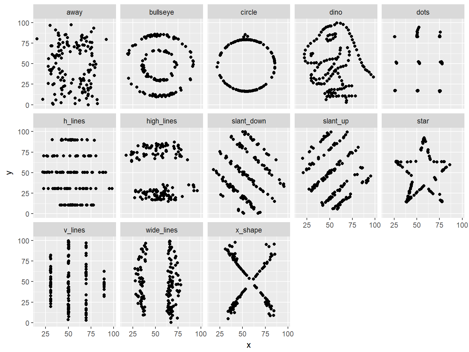

Use case - integration

library(reticulate)
os <- import("os")
os$getcwd()

## [1] "T:\\sites\\superbuild\\pres-r\\pres"

R for data manipulation

Tidyverse

Lots of data sources and destinations
SQL-ish functions
Kicks SQLs butt
“Piping” for easy to read code

I/O packages

readr for flat files
readxl for Excel
haven for SAS, Stata, etc
odbc for databases
jsonlite for JSON
xml2 for XML
httr for APIs
rvest for web scraping
sparklyr for Spark

Data manipulation packages

dplyr for “SQL”
dbplyr for “SQL” against DBs
tidyr for pivoting and unpivoting data
purrr for loop(ish) stuff without the loops
magrittr for pipelines

Bulk read example

list.files("../demo/multiread", full.names = TRUE) %>% map_df(read_csv, 
    col_types = cols(.default = col_character()))

## # A tibble: 105 x 7
##    Timestamp  `Your first name` `Your favourite i~ `Your pet's name (with~
##    <chr>      <chr>             <chr>              <chr>                  
##  1 15/06/201~ Maëlle            Dulce de leche     <NA>                   
##  2 15/06/201~ Dave              Lemon              Cally                  
##  3 15/06/201~ Ahmadou           Caramel            Tigrou                 
##  4 15/06/201~ Arun              Strawberry         Zeus                   
##  5 15/06/201~ Ed                Peach              Charlie                
##  6 15/06/201~ Kyle              Blueberry          Nemo                   
##  7 15/06/201~ Lilian            raspberry          <NA>                   
##  8 15/06/201~ Bea               lemon              peppers                
##  9 15/06/201~ Fred              cookie dough       Max                    
## 10 15/06/201~ David             Vanilla            Jesus                  
## # ... with 95 more rows, and 3 more variables: `The number of
## #   floor/stories your residence has` <chr>, `The year you were born in
## #   (YYYY)` <chr>, `Your favourite day of the week` <chr>

Data pipelines

starwars %>% unite(homeworld_species, homeworld, species) %>% 
    count(homeworld_species)

## # A tibble: 58 x 2
##    homeworld_species            n
##    <chr>                    <int>
##  1 Alderaan_Human               3
##  2 Aleen Minor_Aleena           1
##  3 Bespin_Human                 1
##  4 Bestine IV_Human             1
##  5 Cato Neimoidia_Neimodian     1
##  6 Cerea_Cerean                 1
##  7 Champala_Chagrian            1
##  8 Chandrila_Human              1
##  9 Concord Dawn_Human           1
## 10 Corellia_Human               2
## # ... with 48 more rows

Databases

library(DBI)
library(odbc)

driver = "ODBC Driver 13 for SQL Server"
server = "mhknbn2kdz.database.windows.net"
database = "AdventureWorks2012"
uid = "sqlfamily"
pwd = "sqlf@m1ly"

dbConn <- dbConnect(odbc(), driver = driver, server = server, 
    database = database, uid = uid, pwd = pwd)

Querying databases

library(dbplyr)

medalist <- tbl(dbConn, in_schema("olympics", "medalist"))
sport <- tbl(dbConn, in_schema("olympics", "sport"))

medalist %>% left_join(sport)

## Joining, by = "SportID"

## # Source:   lazy query [?? x 12]
## # Database: Microsoft SQL Server
## #   12.00.0600[sqlfamily@mhknbn2kdz/AdventureWorks2012]
##    MedalistID Event  Edition Athlete  NOC   Gender Medal Season MedalValue
##         <int> <chr>    <int> <chr>    <chr> <chr>  <chr> <chr>       <dbl>
##  1          1 1500m~    1900 HALMAY,~ HUN   Men    Bron~ Summer          3
##  2          2 1500m~    1900 JARVIS,~ GBR   Men    Gold  Summer          1
##  3          3 1500m~    1900 WAHLE, ~ AUT   Men    Silv~ Summer          2
##  4          4 200m ~    1900 DROST, ~ NED   Men    Bron~ Summer          3
##  5          5 200m ~    1900 HOPPENB~ GER   Men    Gold  Summer          1
##  6          6 200m ~    1900 RUBERL,~ AUT   Men    Silv~ Summer          2
##  7          7 200m ~    1900 HALMAY,~ HUN   Men    Silv~ Summer          2
##  8          8 200m ~    1900 RUBERL,~ AUT   Men    Bron~ Summer          3
##  9          9 200m ~    1900 LANE, F~ AUS   Men    Gold  Summer          1
## 10         10 200m ~    1900 KEMP, P~ GBR   Men    Bron~ Summer          3
## # ... with more rows, and 3 more variables: DisciplineID <int>,
## #   SportID <int>, Sport <chr>

R for data visualisation

Key packages

ggplot2 for static viz
- ggthemes for extra themes
- ggraph for graph viz in ggplot
- ggmap for geospatial in ggplot
plotly for interactive viz
htmlwidgets for generating anything html / javascript
DiagrammeR for flowcharts and things

ggplot2 basics

ggplot(datasaurus_dozen, aes(x, y)) + geom_point() + facet_wrap(~dataset, 
    ncol = 5)

Turning a ggplot interactive

library(plotly, quietly = TRUE)
p <- ggplot(datasaurus_dozen, aes(x, y)) + geom_point() + facet_wrap(~dataset, 
    ncol = 5)
ggplotly(p)

## We recommend that you use the dev version of ggplot2 with `ggplotly()`
## Install it with: `devtools::install_github('hadley/ggplot2')`

Building interactive plots

map_data("world", "UK") %>% group_by(group) %>% plot_geo(x = ~long, 
    y = ~lat) %>% add_markers(size = I(1))

R for reporting

Key packages

rmarkdown for using markdown
knitr for converting R markdown files to other formats
revealjs for whizzy presentations
bookdown for making books
blogdown for sites
officer for complex(ish) Word and PowerPoint
shiny for interactive reports
flexdashboard for dashboards
DataExplorer for quick reports on data

rmarkdown & revealjs

See slide source code!

bookdown

See Data Manipulation in R source code

shiny & flexdashboard

See Cost of Coffee app & source code

DataExplorer

DataExplorer::create_report(who)

Nifty stuff

Plays well with others

Consume Python & JS
Consume from Python & JS
Incoporated into many BI platforms
Run in-database
Run in Spark

Community

R UGs
R Ladies
Conferences e.g. SatRday Cardiff June 23rd
Twitter (#rstats)
r-bloggers.com
r-weekly.com

Intro to R

Steph Locke @theStephLocke Locke Data

2018-06-29

Setup

Steph Locke

Agenda

R

R

Use case - wrangling data

Use case - visualisation

Use case - integration

R for data manipulation

Tidyverse

I/O packages

Data manipulation packages

Bulk read example

Data pipelines

Databases

Querying databases

R for data visualisation

Key packages

ggplot2 basics

Turning a ggplot interactive

Building interactive plots

R for reporting

Key packages

rmarkdown & revealjs

bookdown

shiny & flexdashboard

DataExplorer

Nifty stuff

Plays well with others

Community

Next steps

Q&A

Learn

Follow up with me