Simpsons Paradox data

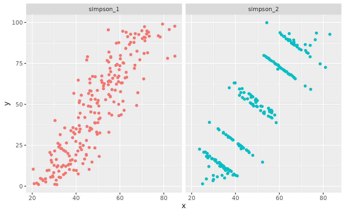
A dataset demonstrating Simpson's Paradox with a strongly positively correlated dataset (simpson_1) and a dataset with the same positive correlation as simpson_1, but where individual groups have a strong negative correlation (simpson_2).

Usage

simpsons_paradox

Format

A data frame with 444 rows and 3 variables:

• dataset: indicates which of the two datasets the data are from, simpson_1 or simpson_2

• x: x-values

• y: y-values

References

Matejka, J., & Fitzmaurice, G. (2017). Same Stats, Different Graphs: Generating Datasets with Varied Appearance and Identical Statistics through Simulated Annealing. CHI 2017 Conference proceedings: ACM SIGCHI Conference on Human Factors in Computing Systems. Retrieved from https://www.autodeskresearch.com/publications/samestats.

Examples

if(require(ggplot2)){
  ggplot(simpsons_paradox, aes(x=x, y=y, colour=dataset))+
    geom_point()+
    theme(legend.position = "none")+
    facet_wrap(~dataset, ncol=3)
}


# Base R Plots
state <- par('mfrow')

par(mfrow = c(1, 2))

sets <- unique(datasaurus_dozen$dataset)

for (i in 1:2) {
  df <- simpsons_paradox[simpsons_paradox$dataset == paste0('simpson_', i), ]
  plot(df$x, df$y, pch = 16, xlab = '', ylab = '')
  title(paste0('Simpson\'s Paradox ', i))
}


par(state)
#> NULL