Data Science Fundamentals
Steph Locke
2018-09-01
Agenda
- Business challenge
- Process
- Data & EDA
- Sampling
- Modelling
- Evaluation
- Operationalising
- Monitoring
Steph Locke & Locke Data
- Steph
- MVP
- Learn R books: geni.us/rfundamentals
- Locke Data
- Consultancy focussed on helping organisations get started with data science
- @thestephlocke @lockedata
- steph@itsalocke.com
- itsalocke.com
Business Challenge
Business Challenge/goal
- Increase customer profitability
- Increase quantity of customers
- Reduce overheads
Data science challenge
Find the lever you can push on to change behaviours that helps with business goal.
Getting started
Tips
- Pick something only somewhat important and valuable to begin
- Find many levers
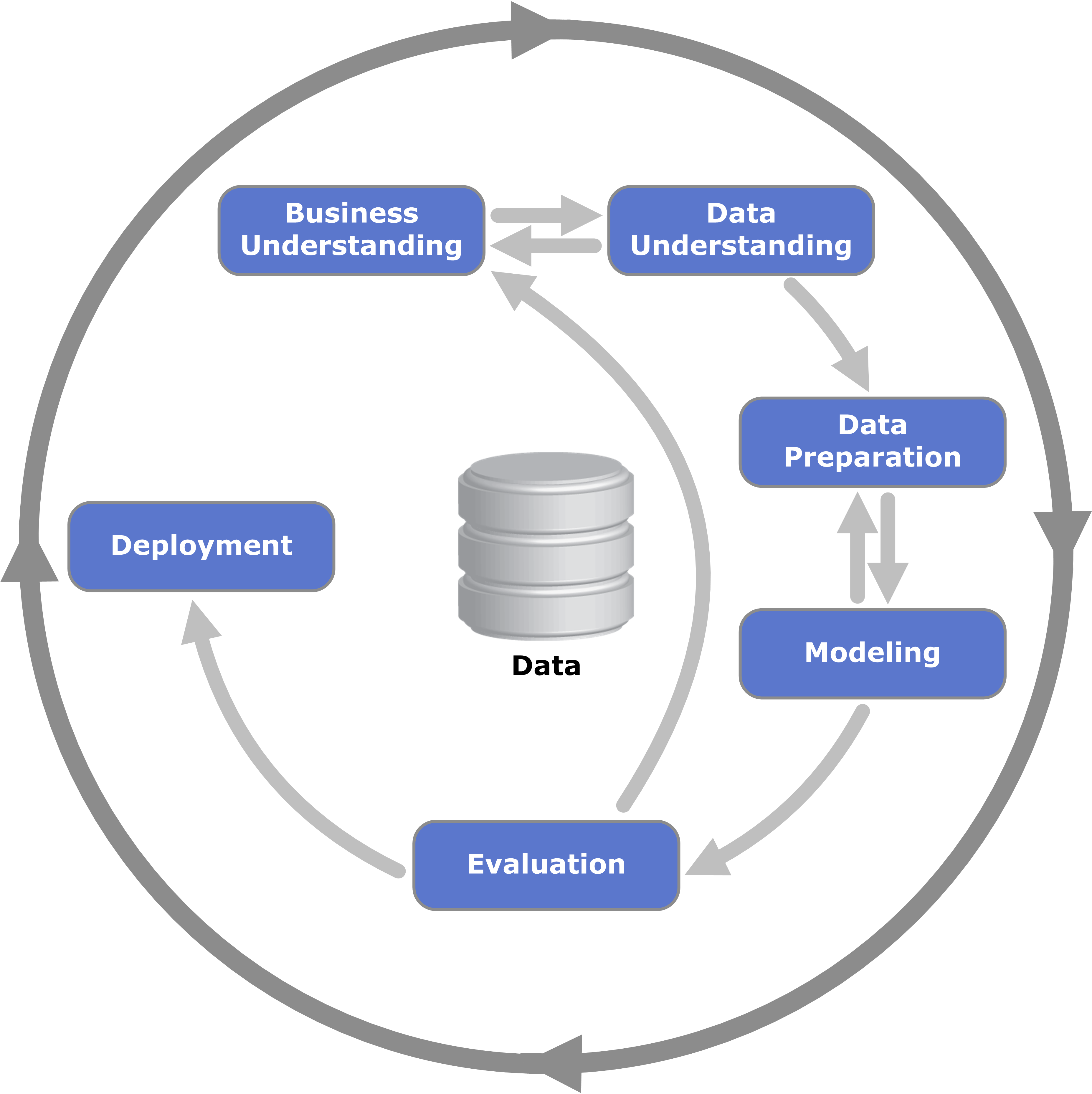
Process
CRISP-DM
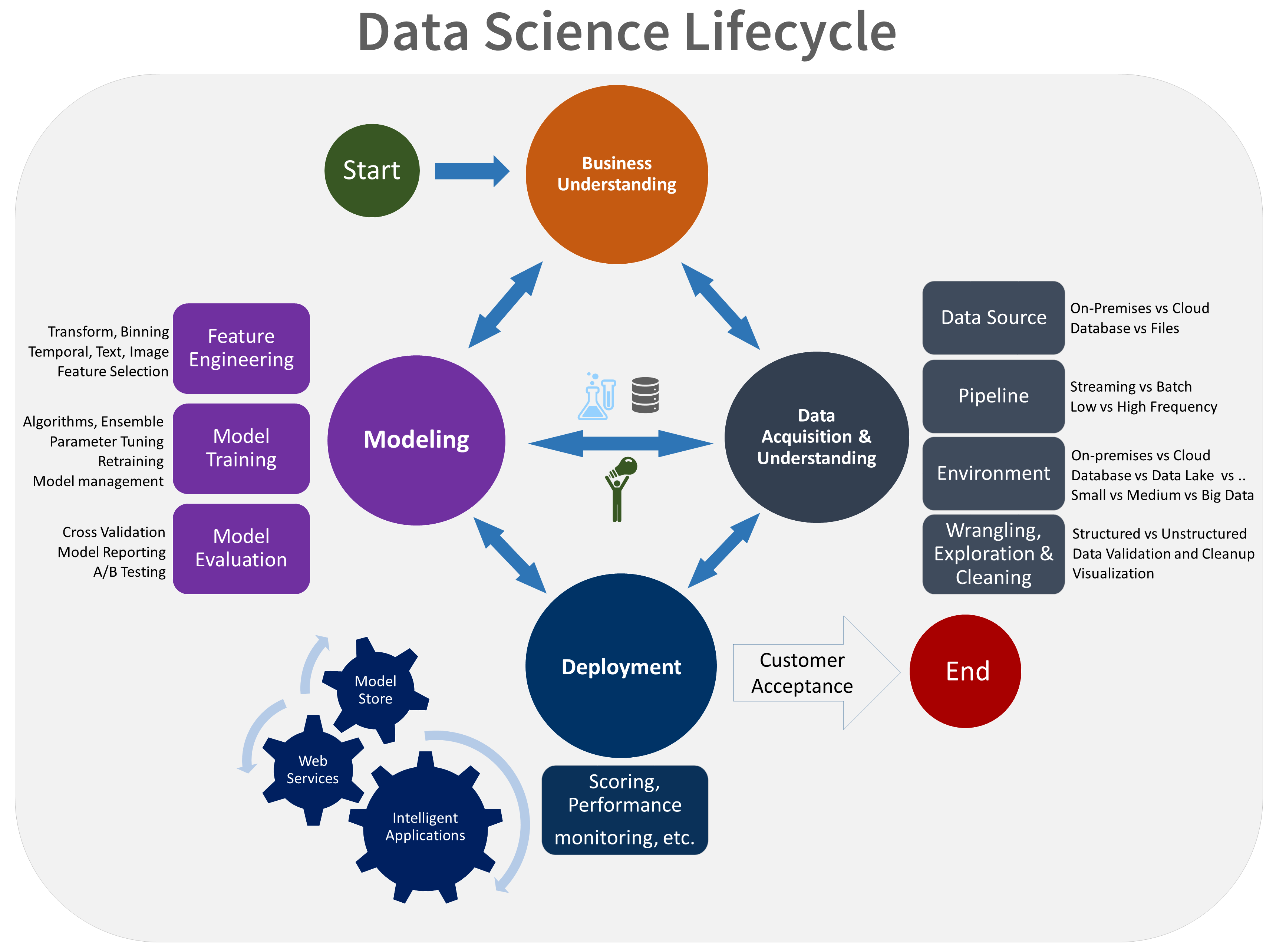
Team Data Science process
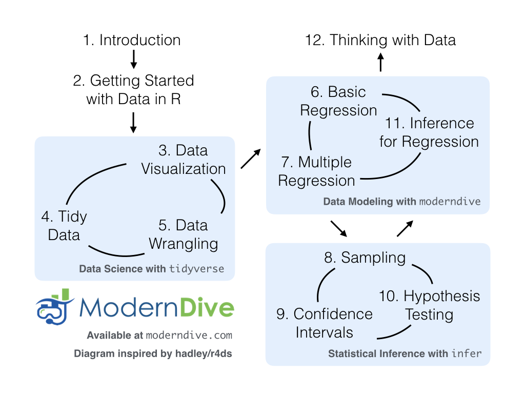
Data science routes
Getting started
Tips
- Iterate
- Prototype
Next steps
- Check out Experiment kanban
- Check out MSFT data science process
Data & EDA
Data
- Do you have enough data?
- What biases are in the data that you might end up reinforcing?
- Have there been changes over time that mean the information means different things?
- Does it actually measure what you think it’s measuring?
Extra data
- Where can you get extra information from?
- Do the join criteria work?
- Will you be able to get it for production purposes?
Exploration
- Analyse the heck out of that data!
- Create extra “features”
Visualisation
Getting started
Tips
- Data dictionaries
- Code everything
Next steps
- Read R for Data Science geni.us/rfords
- Use your existing tools
Example code
library(DBI)
library(odbc)

driver   = "ODBC Driver 13 for SQL Server"
server = "lockedata2.westeurope.cloudapp.azure.com"
database = "datasci"
uid = "lockedata"
pwd = "zll+.?=g8JA11111"


dbConn<-dbConnect(odbc(),
          driver=driver, server=server,
          database=database, uid=uid,
          pwd=pwd)
Example code
library(tidyverse)
library(dbplyr)

flights<-tbl(dbConn,"flights")
carriers<-tbl(dbConn,"flights_carriers")

flights %>%
  inner_join(carriers)
## # Source:   lazy query [?? x 20]
## # Database: Microsoft SQL Server 14.00.3015[dbo@lockedata2/datasci]
##     year month   day dep_time sched_dep_time dep_delay arr_time
##    <int> <int> <int>    <int>          <int>     <dbl>    <int>
##  1  2013     5    30     1434           1435        -1     1545
##  2  2013     5    30     1441           1445        -4     1546
##  3  2013     5    30     1448           1455        -7     1607
##  4  2013     5    30     1455           1459        -4     1614
##  5  2013     5    30     1455           1459        -4     1609
##  6  2013     5    30     1521           1530        -9     1735
##  7  2013     5    30     1529           1530        -1     1832
##  8  2013     5    30     1551           1600        -9     1652
##  9  2013     5    30     1604           1610        -6     1749
## 10  2013     5    30     1604           1608        -4     1727
## # ... with more rows, and 13 more variables: sched_arr_time <int>,
## #   arr_delay <dbl>, carrier <chr>, flight <int>, tailnum <chr>,
## #   origin <chr>, dest <chr>, air_time <dbl>, distance <dbl>, hour <dbl>,
## #   minute <dbl>, time_hour <dttm>, name <chr>
Example code
library(DataExplorer)
flights %>%
  collect %>%
  create_report()
Sampling
Sampling basics
- [OPTIONAL] Dataset for missing data
- Dataset for building your model
- Dataset for testing your model
Considerations
- Balanced or unbalanced
- Bootstrapping
Getting started
Tips
- Make samples reproducible
- Don’t double-dip!
Next steps
- Read about sampling
Example code
library(rsample)
flights %>%
  initial_split()  ->
  samples

nrow(training(samples))
nrow(testing(samples))
## [1] 252582
## [1] 84194Modelling
Models
- Supervised vs unsupervised
- Parametric vs non-parametric
Models
- Regression
- Trees
- Others
Candidate models
- Simple model
- Complex model
- Different model types
Getting started
Tips
- Models are cattle not pets
Next steps
- Check out setosa.io
Example code
samples %>%
  training() %>%
  lm(arr_delay ~ as.factor(month) + as.factor(day) + hour , data=.) ->
  initial_lm

initial_lm
##
## Call:
## lm(formula = arr_delay ~ as.factor(month) + as.factor(day) +
##     hour, data = .)
##
## Coefficients:
##        (Intercept)   as.factor(month)2   as.factor(month)3
##         -15.578026           -0.523332           -0.009617
##  as.factor(month)4   as.factor(month)5   as.factor(month)6
##           4.925857           -2.322463           10.916768
##  as.factor(month)7   as.factor(month)8   as.factor(month)9
##          10.579558            0.350634          -10.001152
## as.factor(month)10  as.factor(month)11  as.factor(month)12
##          -6.282354           -5.779870            9.156317
##    as.factor(day)2     as.factor(day)3     as.factor(day)4
##          -0.835973           -3.053353           -9.091525
##    as.factor(day)5     as.factor(day)6     as.factor(day)7
##          -6.589357           -8.952260            2.497260
##    as.factor(day)8     as.factor(day)9    as.factor(day)10
##          11.810864            1.294906            7.777381
##   as.factor(day)11    as.factor(day)12    as.factor(day)13
##           2.998162            3.405094            2.031710
##   as.factor(day)14    as.factor(day)15    as.factor(day)16
##          -4.301413           -8.459728           -3.757981
##   as.factor(day)17    as.factor(day)18    as.factor(day)19
##           2.303175            2.975389            3.165694
##   as.factor(day)20    as.factor(day)21    as.factor(day)22
##          -5.861942           -4.406458           10.942822
##   as.factor(day)23    as.factor(day)24    as.factor(day)25
##           9.586899            3.568447            2.930465
##   as.factor(day)26    as.factor(day)27    as.factor(day)28
##          -3.970729           -3.841386            1.254968
##   as.factor(day)29    as.factor(day)30    as.factor(day)31
##          -7.937313           -6.378870           -4.457317
##               hour
##           1.667757
Evaluation
Critical Success Factors
- False positives vs false negatives
- Ranking
- Aligns with experts
Data diving
- Segments
- Structural weaknesses
- Test data
Getting started
Tips
- Don’t just rely on single metric
Example code
library(broom)
initial_lm %>%
  glance()
## # A tibble: 1 x 11
##   r.squared adj.r.squared sigma statistic p.value    df  logLik    AIC
## *     <dbl>         <dbl> <dbl>     <dbl>   <dbl> <int>   <dbl>  <dbl>
## 1    0.0680        0.0679  43.0      427.       0    43 -1.27e6 2.54e6
## # ... with 3 more variables: BIC <dbl>, deviance <dbl>, df.residual <int>
Operationalising
Features
- ETL for new data and calculations
- What data quality stuff had to be done?
Model
- How will you store the model?
- Does it need versioning?
- When will it need to be updated and how?
Technology
- What’s the easiest way of getting live?
- What’s the long term way of getting it live?
- What’s your “bus factor”?
Getting started
Tips
- KISS
- Operationalising a model often takes longer than the modelling exercise (at least initially)
Next steps
- Check out R in SQL Server
- Check out Azure ML
Monitoring
Logging
- Log results
- Log all the things
Metrics
- Measure the business lever & other KPIs
- Set tolerances for negative impacts on other metrics
- J-performance
Holdouts
- Always have a control group
Getting started
Tips
- Plan for monitoring, don’t make it an after-thought
Conclusion
Process
Tips
- Pick something only somewhat important and valuable to begin
- Find many levers
- Iterate
- Prototype
- Data dictionaries
- Code everything
- Make samples reproducible
- Don’t double-dip!
Tips
- Models are cattle not pets
- Don’t just rely on single metric
- KISS
- Operationalising a model often takes longer than the modelling exercise (at least initially)
- Plan for monitoring, don’t make it an after-thought
Follow up
- @thestephlocke @lockedata
- steph@itsalocke.com
- itsalocke.com/talks